flowchart TD
A[Data] --> B[population data]
A --> C[smoking data]
C --> D[[reclassify directorate names to regions]] --> E[[calculate age bands]] --> F[[calculate smoking counts]]
B --> G[[calculate age bands]] --> H[[calculate population counts]]
H --> I[[join datasets]]
F --> I
I --> J[calculate rates and ci]
8 Smoking
8.1 Workflow
8.1.1 Load census population and create age bands
Code
## create age band

pops <- setDT(pops)[, `:=` (`18-44`  = dplyr::between(age, 18, 44), `15+` = age >= 15, `80+` = age >= 80, age_band = cut(age, seq(0, 110, 5), right = FALSE))][]

pop_age <- pops[, .(n = .N, sumpops = sum(Population, na.rm = TRUE)), by = .(Region, age_band,  Gender)][order(age_band)]

pop1844F <- pops[, .(n = .N, sumpops = sum(Population, na.rm = TRUE)), by = .(Region, `18-44`,  Gender)][`18-44` == "TRUE" & Gender == "Female",]

pop15F <- pops[, .(n = .N, sumpops = sum(Population, na.rm = TRUE)), by = .(Region, `15+`,  Gender)][`15+` == "TRUE" & Gender == "Female",]
8.1.2 Load smoking data and calculate age bands
Note: it is not clear if the dummy data is a random sample of clinic attendance data.
Code
smok_age <- smoking[, `:=` (`18-44`  = dplyr::between(age, 18, 44), `15+` = age >= 15, `80+` = age >= 80, age_band = cut(age, seq(0, 110, 5), right = FALSE))][]

smok_age_bands <- smok_age[, .(n = .N, smokers = sum(n, na.rm = TRUE)), by = .(Region, age_band,  Gender)][order(age_band)]

smok1844F <- smok_age[, .(n = .N, smokers = sum(n, na.rm = TRUE)), by = .(Region, `18-44`,  Gender)][`18-44` == "TRUE" & Gender == "female",]

smok15F <- smok_age[, .(n = .N, smokers = sum(n, na.rm = TRUE)), by = .(Region, `15+`,  Gender)][`15+` == "TRUE" & Gender == "female",]
8.1.3 Join datasets and calculate rates
This step uses Byar’s method for confidence interval for rates
Code
smok_rates <- pop1844F |>
    left_join(smok1844F, by = "Region") |>
    phe_rate(x = smokers, n = sumpops)

smok_rates |>
    dplyr::select(Region, smokers, population = sumpops, value, lowercl, uppercl) |>
    flextable::flextable()
Region | smokers | population | value | lowercl | uppercl |
|---|---|---|---|---|---|
'Asir | 366,324 | ||||
Al Bahah | 28 | 61,969 | 45.183882 | 30.017729 | 65.30573 |
Al Hudud ash Shamaliyah | 4 | 70,149 | 5.702148 | 1.553643 | 14.59976 |
Al Jawf | 23 | 103,536 | 22.214495 | 14.077587 | 33.33412 |
Al Madinah al Munawwarah | 387,944 | ||||
Al Mintaqah ash Sharqiyah | 877,403 | ||||
Al Qasim | 249,081 | ||||
Ar Riyadh | 1,609,493 | ||||
Ha'il | 22 | 136,642 | 16.100467 | 10.086571 | 24.37741 |
Jazan | 267,342 | ||||
Makkah al Mukarramah | 1,507,301 | ||||
Najran | 82 | 105,915 | 77.420573 | 61.572876 | 96.10050 |
Tabuk | 291 | 163,453 | 178.032829 | 158.162585 | 199.70848 |
Code
smok_rates |>
    write_csv("data/smok_rates.csv")

smok_rates |>
    ggplot() +
    geom_col(aes(reorder(Region, value), value)) +
    geom_linerange(aes(x = Region, ymin = lowercl, ymax = uppercl)) +
    coord_flip() +
    labs(x = " ",
         y = "Rate per 100.000")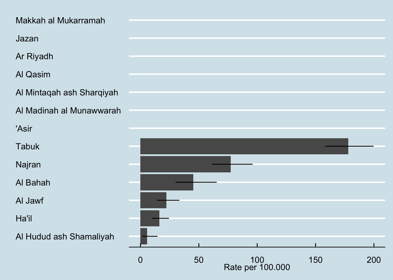
8.1.4 Age-specific attendance rates
Code
smok_age_agg <- smok_age_bands[, .(tot_smokers = sum(smokers)), by = .(age_band, Gender)][]

options(scipen = 999, digitds = 2)

## m:f as smoking ratios

smok_rates_gender <- pop_age |>
    dplyr::select(-Region) |>
    mutate(Gender = recode(Gender, "Female" = "female", "Male" = "male")) |>
    left_join(smok_age_agg, by = c("age_band", "Gender")) |>
    group_by(age_band, Gender) |>
    reframe(nat_smok = sum(tot_smokers, na.rm = TRUE),
           nat_pop = sum(sumpops)) |>
    phe_rate(x = nat_smok, n = nat_pop) |>
    mutate(value = ifelse(Gender == "female", -value, value)) |>
    ggplot() +
    geom_col(aes(age_band, value, fill = Gender)) +
    coord_flip() +
    scale_fill_manual(values = c("blue", "red")) +
    labs(x = "",  y = "Attendance rate per 100000")

smok_rates_gender 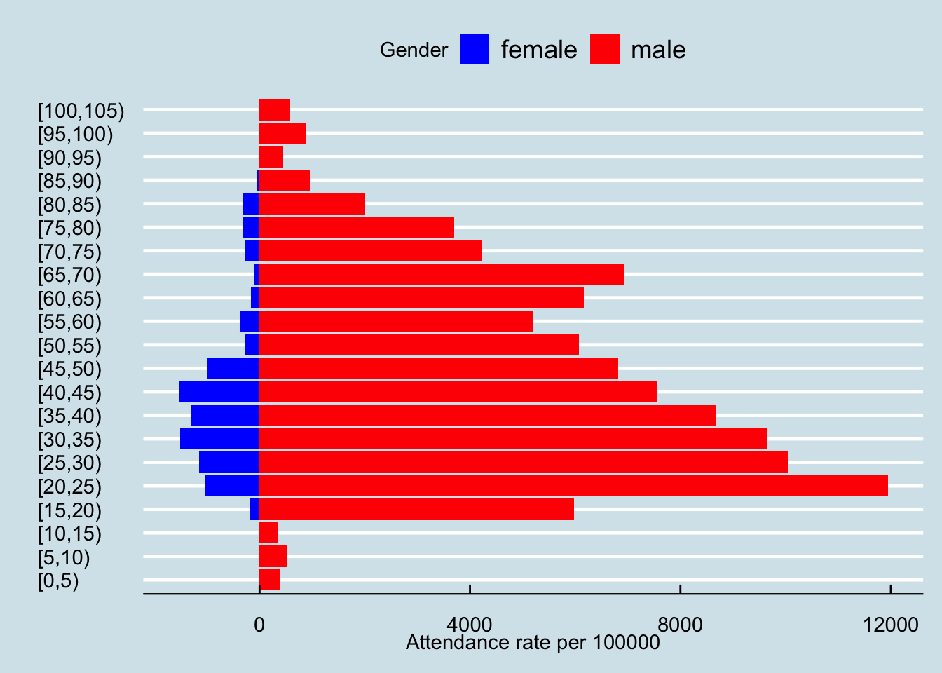
Code
smok_gender_ratio <- pop_age |>
    dplyr::select(-Region) |>
    mutate(Gender = recode(Gender, "Female" = "female", "Male" = "male")) |>
    left_join(smok_age_agg, by = c("age_band", "Gender")) |>
    group_by(age_band, Gender) |>
    reframe(nat_smok = sum(tot_smokers, na.rm = TRUE),
           nat_pop = sum(sumpops)) |>
    phe_rate(x = nat_smok, n = nat_pop) |>
    slice(7:36) |>
    group_by(age_band) |>
    reframe(ratio = value[2] / value[1]) |>
    mutate(mean_ratio = mean(ratio))
The relative attendance rate for males is 17.32 times that of females. Smoking clinic attendance rates could be used as a proxy for population smoking rates if the relationship between attendance and prevalence is known . For example, survey data suggests that KSA male smoking rates are around 20% which implies a female smoking rate based on 1.15%. In fact, available survey data (Algabbani et al. (2018)), and estimates from the Global Burden of Disease ((“Prevalence of Smoking,” n.d.; Xiang et al. 2023)), suggest a smoking prevalence in females over 15 of 2%,