Code
ksa_bound |>
ggplot() +
geom_sf()
mapview(ksa_bound)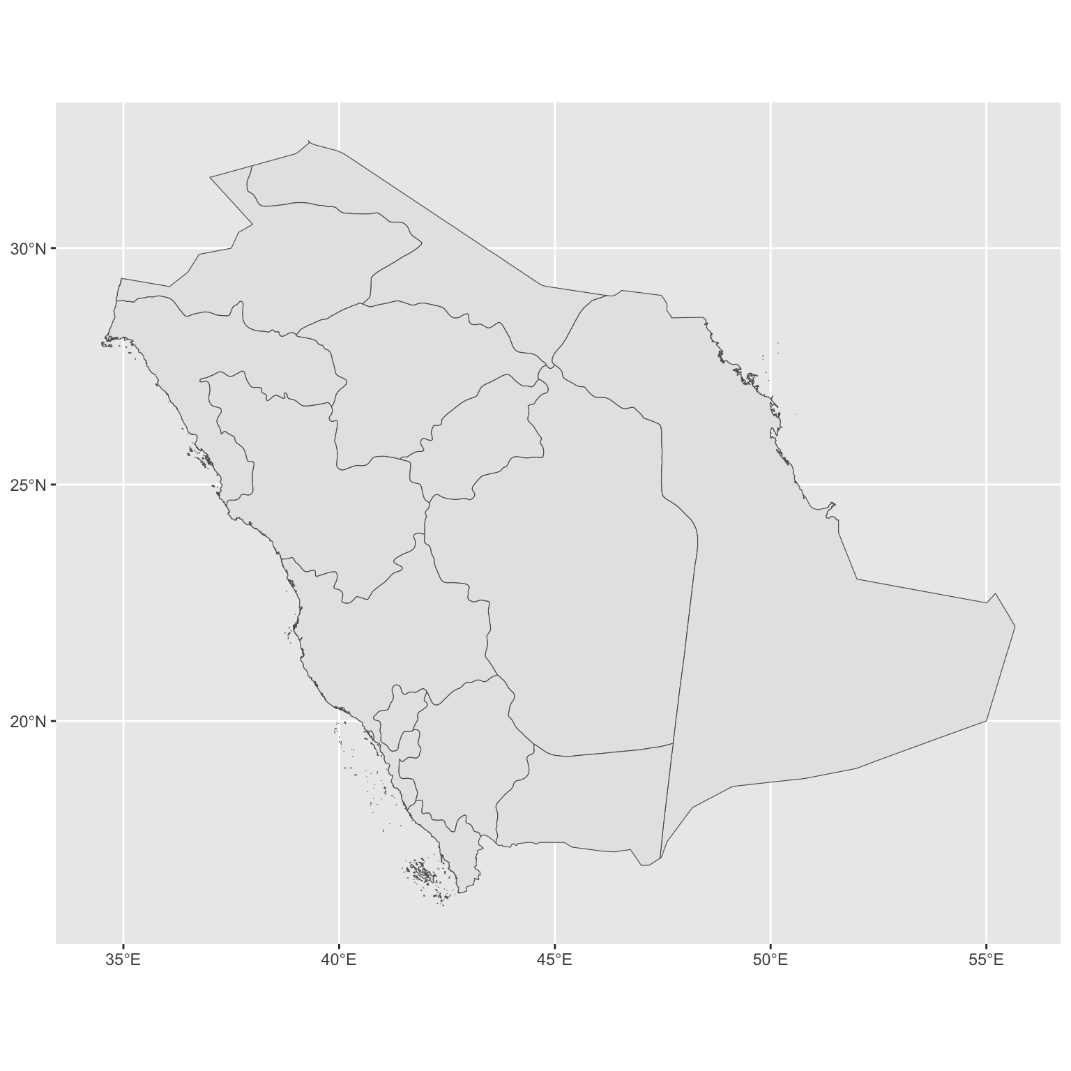
Maps
A regional boundary file is downloaded as part of the data pre-processing step and is contained in the object sa_bound.
This can be plotted as a static or interactive map:
ksa_bound |>
ggplot() +
geom_sf()
mapview(ksa_bound)Attribute data (e..g area rates) needs to be combined with the boundary data in order to map them. Taking the example of injury….
inj <- read_csv("data/injury_dsr.csv")setdiff(inj$region, ksa_bound$ADM1_EN)[1] "'Asir" "Al Madinah al Munawwarah"
[3] "Al Mintaqah ash Sharqiyah" "Al Qasim"
[5] "Ar Riyadh" "Jazan"
[7] "Makkah al Mukarramah" ksa_bound$ADM1_EN [1] "`Asir" "Al Bahah"
[3] "Al Hudud ash Shamaliyah" "Al Jawf"
[5] "Al Madinah" "Al Quassim"
[7] "Ar Riyad" "Ash Sharqiyah"
[9] "Ha'il" "Jizan"
[11] "Makkah" "Najran"
[13] "Tabuk" ## recode area names and join to boundary data
inj_sf <- inj |>
mutate(region1 = recode(region,
"'Asir" = "`Asir",
"Al Madinah al Munawwarah" = "Al Madinah",
"Al Qasim" = "Al Quassim",
"Makkah al Mukarramah" = "Makkah",
"Al Mintaqah ash Sharqiyah" = "Ash Sharqiyah",
"Ar Riyadh" = "Ar Riyad",
"Jazan" = "Jizan"),
region1 = ifelse(region1 != region, region1, region)
)
inj_sf <- left_join(ksa_bound, inj_sf, by = c("ADM1_EN" = "region1"))
inj_sf |>
filter(is.na(gender))Simple feature collection with 1 feature and 19 fields
Geometry type: MULTIPOLYGON
Dimension: XY
Bounding box: xmin: 34.4943 ymin: 24.53653 xmax: 40.17387 ymax: 28.98889
Geodetic CRS: WGS 84
# A tibble: 1 × 20
gml_id Shape_Leng Shape_Area ADM1_EN ADM1_PCODE ADM1_REF ADM1ALT1EN ADM1ALT2EN
* <chr> <dbl> <dbl> <chr> <chr> <chr> <chr> <chr>
1 ksa_b… 34.6 9.05 Tabuk SA07 <NA> <NA> <NA>
# ℹ 12 more variables: ADM0_EN <chr>, ADM0_PCODE <chr>, date <date>,
# validOn <date>, validTo <date>, geometryProperty <MULTIPOLYGON [°]>,
# region <chr>, crude.rate <dbl>, adj.rate <dbl>, lci <dbl>, uci <dbl>,
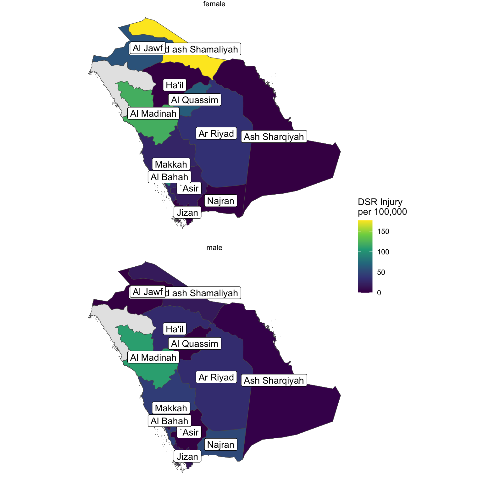
# gender <chr>## convert back to spatial data and plot
inj_sf |> st_as_sf() |>
filter(!is.na(gender)) |>
ggplot() +
geom_sf(data = ksa_bound) +
geom_sf(aes(fill = 100000 * adj.rate)) +
ggplot2::geom_sf_label(aes(label = ADM1_EN)) +
facet_wrap(~ gender, ncol = 1) +
theme_void() +
scale_fill_viridis_c(name = "DSR Injury\nper 100,000")
mapview(inj_sf |> st_as_sf() |>
filter(gender == "female") |> mutate(adj.rate = 100000 * adj.rate), zcol = "adj.rate")